Welcome Back!

In my previous post , I used Google’s Youtube API to collect data from three of my favorite Golf Youtube channels: Good Good Golf, gm_golf, and Bob Does Sports. Our end goal is to determine the factors that contribute to a successful golf Youtube channel. In this post, we will be performing some Exploratory Data Analysis on the data we collected. The github repo for this project can be found here .

Important Note

For all plots generated in the EDA, we will be referring to each channel as the following:

Good Good Golf = GGG
gm_golf = GM
Bob Does Sports = BDS

Function to Save Visualizations Quickly

Disclaimer: this is not relevant to the EDA, but I wanted to include it because I thought it was cool.

I knew I was going to be saving a bunch of plots as images into a different directory, so I used plotly.io in a function that I wrote to save my visualizations. I didn’t want to wait until I was finished with all of my plots, then write a for loop to save them all at once. I wanted something I could use to save my plots to the ‘images’ directory as I was creating them. Here is the function I wrote:

def save_figure(fig, filename):
    """Save the given plotly figure to the specified filename in the images directory."""
    filepath = f'../assets/images/{filename}'
    pio.write_image(fig, filepath)

Where filepath is the path to the ‘images’ directory.

So, for example, if I wanted to save a plot as ‘golf.eda1.png’, I would write:

save_figure(fig, 'golf.eda1.png')

Vuala! ‘golf.eda1.png’ is saved to the ‘images’ directory. EZ PZ.

EDA

The first thing I wanted to do was to get a general idea of how many videos each channel has posted. I created a bar chart to visualize this data:

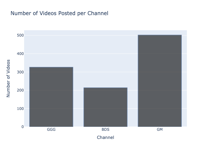
This is the one and only time that I specified rgb values for the colors of my bar chart. I find it much easier to use Plotly’s default colors for my visualizations, which is what I use for the rest of my visualizations. Here is the code for the visualization above:

import plotly.graph_objects as go

fig = go.Figure(data=[go.Bar(
    x=['GGG', 'BDS', 'GM'], 
    y=[len(dfgood), len(dfbob), len(dfgm)]
    )])
fig.update_traces(marker_color='black', marker_line_color='rgb(8,48,107)', marker_line_width=1.5, opacity=0.6)
fig.update_layout(title_text='Number of Videos Posted per Channel')
fig.update_xaxes(title_text='Age Group')
fig.update_yaxes(title_text='Number of Diseases')
fig.write_image("assets/images/golf.eda1.png")
fig.show()

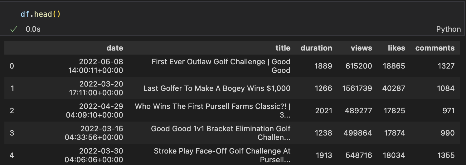
Note: I have the data from each channel saved into separate dataframes.

This visualization was not very informative, as it does not take into account the amount of time that a channel has been active for. To get a better idea of how OFTEN each channel posts, I filtered the data to only include videos that were posted in 2021. Throwback to my previous post, here are the columns that I am working with:

I then created a bar chart to visualize this data:

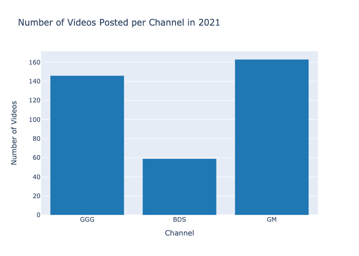
This visualization I used Plotly’s default colors. Since I knew that I would be using Plotly’s default colors for the rest of my visualizations, I imported plotly colors to save time. Here is the code for the visualization above:

import plotly.colors as colors

fig = go.Figure(data=[go.Bar(
    x=['GGG', 'BDS', 'GM'], 
    y=[len(dfgood21), len(dfbob21), len(dfgm21)],
    marker={'color': colors.DEFAULT_PLOTLY_COLORS[0]}
    )])
fig.update_layout(title_text='Number of Videos Posted per Channel in 2021')
fig.update_xaxes(title_text='Channel')
fig.update_yaxes(title_text='Number of Videos')
save_figure(fig, 'golf.eda2.png')
fig.show()

Plotly has 10 default colors that you can use, by setting the figure’s marker color to:

colors.DEFAULT_PLOTLY_COLORS[0:9].

Next I wanted to see a line graph of metrics over time. I decided to knock out all three metrics at once. On one plotly figure, I made three subplots, one for each metric (views, likes, and dislikes). On each subplot, I plotted the data for each channel. First I will talk about the code I used to make this figure, then I will talk about the figure itself.

from plotly.subplots import make_subplots

fig = go.Figure()
fig = make_subplots(rows=3, cols=1, subplot_titles=("Views per Video", "Likes per Video", "Comments per Video"), shared_xaxes=True, vertical_spacing=0.1)
#make the color of each channel be the same for each channel accross sub plots
color = [colors.DEFAULT_PLOTLY_COLORS[2], colors.DEFAULT_PLOTLY_COLORS[4], colors.DEFAULT_PLOTLY_COLORS[9]]
#add the traces for each channel to each subplot without using a loop
fig.add_trace(go.Scatter(x=dfgood['date'], y=dfgood['views'], mode='lines', name='GGG', line_color=color[0]), row=1, col=1)
fig.add_trace(go.Scatter(x=dfbob['date'], y=dfbob['views'], mode='lines', name='BDS', line_color=color[1]), row=1, col=1)
fig.add_trace(go.Scatter(x=dfgm['date'], y=dfgm['views'], mode='lines', name='GM', line_color=color[2]), row=1, col=1)
fig.add_trace(go.Scatter(x=dfgood['date'], y=dfgood['likes'], mode='lines', name='GGG', line_color=color[0]), row=2, col=1)
fig.add_trace(go.Scatter(x=dfbob['date'], y=dfbob['likes'], mode='lines', name='BDS', line_color=color[1]), row=2, col=1)
fig.add_trace(go.Scatter(x=dfgm['date'], y=dfgm['likes'], mode='lines', name='GM', line_color=color[2]), row=2, col=1)
fig.add_trace(go.Scatter(x=dfgood['date'], y=dfgood['comments'], mode='lines', name='GGG', line_color=color[0]), row=3, col=1)
fig.add_trace(go.Scatter(x=dfbob['date'], y=dfbob['comments'], mode='lines', name='BDS', line_color=color[1]), row=3, col=1)
fig.add_trace(go.Scatter(x=dfgm['date'], y=dfgm['comments'], mode='lines', name='GM', line_color=color[2]), row=3, col=1)
fig.update_layout(height=1000, width=1000)
fig.update_xaxes(title_text='Date')
fig.update_traces(showlegend=False)
fig.update_traces(showlegend=True, row=1, col=1)
fig.update_yaxes(title_text='Number of Views', row=1, col=1)
fig.update_yaxes(title_text='Number of Likes', row=2, col=1)
fig.update_yaxes(title_text='Number of Comments', row=3, col=1)
save_figure(fig, 'golf.eda3.png')
fig.show()

This was a lot of code, I assume there is a more efficient way to type all of this out. Let me know if you know of a better way to do this. You can see that I first made 3 subplots. I know that the line graphs will be longer than they are taller, so I made each subplot be one row instead of one column. I also set the title of each subplot in that same line of code. Next, I made a list of the three different colors that will represent each channel. The next part I’m sure there is some way to do more efficiently than I did. I trace that I added was a single line on a single subplot. When doing it this way, you need to specify which subplot this is being applied to by specifying the row and column. By default, the figure will include a legend that includes each legend for each subplot combined into one legend. That means that by default, the legend will repeat the name and color identifier of each channel three times. To counter this, I set showlegend=False for all traces, then set showlegend=True for the first subplot. The rest of the code is self explanatory.

Now we will look at the figure that this produced:

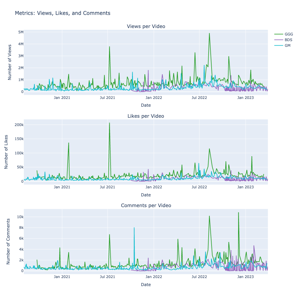
This figure is not very informative. The variability of each metric is too high to see any trends. The high variability causes the yaxes to be so stretched that you can’t see what is going on with the data. It was a nice try, but I will need to find a better way to visualize this data.

I think I can make this figure work if I use a seven day rolling average. I used basically the same code as above, but I used rolling averages instead of the raw data. Here is the code I used to calculate the rolling averages:

# views
dfgood['rolling_views'] = dfgood['views'].rolling(7).mean()
dfbob['rolling_views'] = dfbob['views'].rolling(7).mean()
dfgm['rolling_views'] = dfgm['views'].rolling(7).mean()
# likes
dfgood['rolling_likes'] = dfgood['likes'].rolling(7).mean()
dfbob['rolling_likes'] = dfbob['likes'].rolling(7).mean()
dfgm['rolling_likes'] = dfgm['likes'].rolling(7).mean()
# comments
dfgood['rolling_comments'] = dfgood['comments'].rolling(7).mean()
dfbob['rolling_comments'] = dfbob['comments'].rolling(7).mean()
dfgm['rolling_comments'] = dfgm['comments'].rolling(7).mean()

Here is the plot:

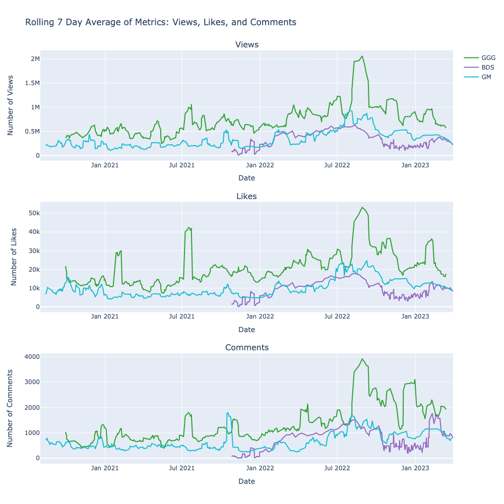
This is much better. I can see that views, likes, and comments all follow similar trends. I think it is a safe assumption that the main driver of these trends are the number of views that a video receives.

I also think that Bob Does Sports has been growing much faster than the other two channels when they first started.

Lastly, I want to see if there is any correlation between the number of views and the duration of the video. I decided to plot three separate figures this time, one for each channel. I wanted to see a scatterplot of the two variables plotted against each other. I also wanted to see the correlation coefficient. To see both, I made the title of each plot using an f-string, and included the calculated correlation coefficient in the title. Here is the code of one of the plots:

cor_good = dfgood['duration'].corr(dfgood['views'])
fig = px.scatter(dfgood, x='duration', y='views')
fig.update_layout(title_text=f'Views vs. Duration: GGG {cor_good}', height=500, width=500)
fig.update_xaxes(title_text='Duration')
fig.update_yaxes(title_text='Number of Views')
save_figure(fig, 'golf.eda5.png')
fig.show()
    

Let’s take a look at the plots:

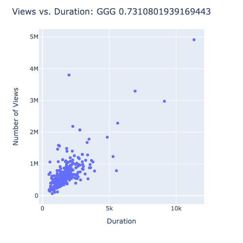
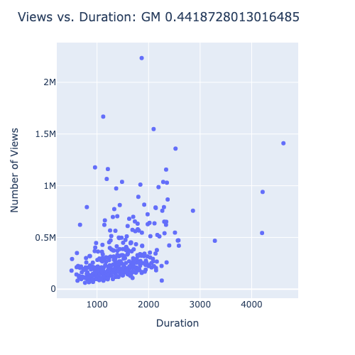
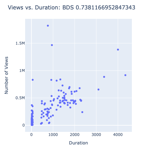
It looks like Good Good has a strong correlation between duration and views. Bob Does Sports had a stronger correlation coefficient, but it appears that is there are a large number of points videos that didn’t get any views. I don’t trust that correlation coefficient as much as I do the one for Good Good. gm_golf has a modest correlation coefficient, but it is not as strong as the other two channels.

Conclusion

After performing some simple EDA on the data, we found that gm_golf and Good Good golf post somewhere around 150 videos per year. Bob Does Sports only posts around 50 videos per year, but they are experiencing a lot of growth. This suggests that upload frequency may not be as important as video quality. We also saw that the number of views, likes, and comments all follow similar trends accross individual channels. It is logical to assume that the number of views is the main driver of these metrics. Lastly, we saw that there is a strong correlation between the duration of a video and the number of views it receives. This suggests that the length of a video is an important factor in determining how many views it will receive.

In our next blog post, we will officially analyze the data and come to a conclusion about our research question.