Machine Learning vs. Deep Learning on Tabular Data

The repository for this project can be found here.

Modern Machine Learning

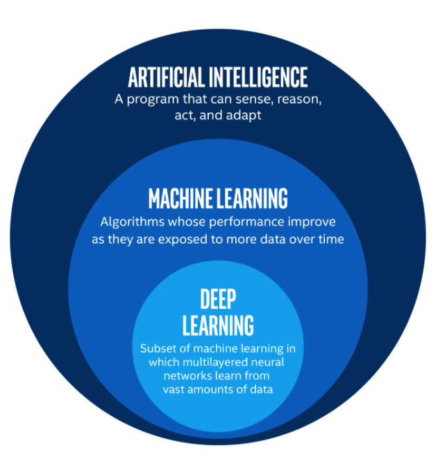
In this age of AI, transformers and other neural network architectures are all the rage. ChatGPT acted as a catalyst to the hype around large language models (LLMs), image generation models, and other complex systems. When it comes to these complex AI systems that we see today, almost all of them are built using complex deep learning architectures. Deep learning is a sub-category of machine learning, and uses multiple layers of neural networks to learn from data.

Deep learning has proved to be a powerful tool in AI, but it has its limitations. One such limitation is that deep learning has historically performed worse on tabular data when compared to traditional machine learning models. I aim to address that limitation in this project, as well as introduce my PyTorch deep learning code base that I have created.

My Background with Deep Learning and Tabular Data

This last summer, I spent my time working at a quantitative hedge fund. We used deep learning models to recommend trades to our portfolio manager. There was a team for multimodal deep learning (models that use multiple modalilties of data. For example, a model that uses text, images, and tabular data), but I was assigned to the tabular models. Our team’s philosophy was that deep learning could outperform traditional machine learning models no matter what modality of data we were using. The stock market is the closest thing that I know of to a chaotic system, and their belief in deep learning came from the idea that we needed a more complex model to capture the complexity of the market.

Deep Learning on Tabular Data

Our tabular data that we used at the hedge fund had thousands of variables and millions of rows. This is ideal when trying to capture complex relationships using deep learning. This, however, is rarely the case with tabular data. Deep learning models are data hungry, and are often too complex for small datasets. I aim to test how well deep learning performs on tabular data when compared to traditional machine learning models.

Model Selection

I am going to use two traditional machine learning models, and one custom deep learning model. The traditional machine learning models that I will be using are XGBoost (gradient boosted tree model) and K Nearest Neighbors. The deep learning model that I will be using will have many layers, and it will use uncertainty calibration.

Uncertainty Calibration

One of the advantages of deep learning models is that they can output uncertainty. This is useful in many applications, such as self-driving cars. If a self-driving car is unsure about what it is seeing, it can output a high uncertainty score. This uncertainty score can then be used to determine if the car should stop or not. This is a very useful feature, but it is not unique to deep learning models. There are many traditional machine learning models that can output uncertainty scores. At the hedge fund, uncertainty calibration was the method that I saw had the biggest impact on the models. I aim to use this method to improve the performance of my deep learning model on tabular data.

About the Data

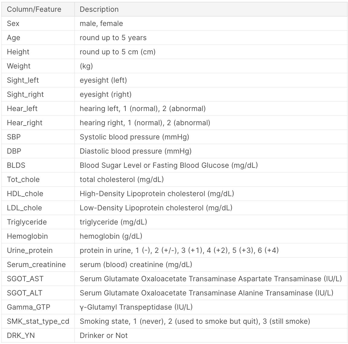
The data I am using is the Smoking and Drinking Dataset with body signal from kaggle. The data contains 991,346 rows, 991,320 rows after removing nulls. There are 23 features: - 1 categorical, 22 numerical. The task that I am trying to predict is whether or not a person drinks, which is a binary classification task. The data is balanced, with 50% of people being drinkers and 50% being non-drinkers. The license for the data is posted on kaggle, and states that the data is free to use for any purpose. The information about each feature is shown below:

Exploratory Data Analysis

Data Exploration

I started my exploration by using one of my favorite libraries: YData Profiling. This library quickly and automatically generates descriptive statistics, data type information, missing value analysis, and distribution visualizations for each column in your dataset. This library also offers advanced features like correlation analysis, unique value counts, and data quality assessments. YData was able to generate the dashboard in 1 minute and 11 seconds. Using the YData report I was able to see that there were 26 rows of duplicates, and no missing values.

Instead of having to set up a loop to show me heatmaps, correlation plots between variables, and other visualizations, YData has all of those plots readily available. This is a great tool for data exploration, and I highly recommend it. To find out more about this library, you can visit their website.

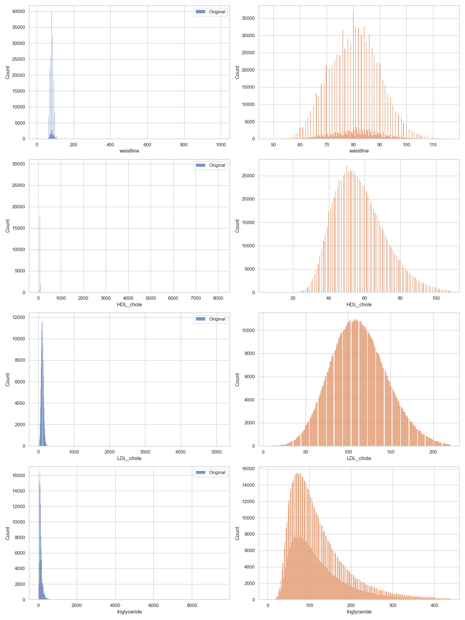
We can see in the YData report that multiple columns such as waistline, HDL_chole, LDL_chole, and triglyceride have significant outliers, and are heavily skewed.

Removing Outliers from the Training Data

My traditional machine learning models are much closer to parametric than my deep learning models. This means that outliers will affect them more than my deep learning models. I will remove outliers from my training data for both my ML and DL models, for continuity sake.

To remove outliers, I used the z-score method. I could have used the IQR method, but I felt that it was not robust-enough. I used a z-score threshold of 3, meaning that any data point that was 3 standard deviations away from the mean was removed. I chose this threshold because I felt that it was a good balance between removing outliers and removing too much data. This process removed 87,291 from the training data, taking it from 991,320 rows to 904,029.

I then compared the before and after distributions of all 18 numeric variables for a visual check. Here are the four variables mentioned before that had outliers (blue is before outliers were removed, orange is after):

Baseline Models

To get an idea of what kind of performance I can expect from my models, I implemented a logistic regression model and a SVM model. Both of these models were not tuned at all, I used the default hyperparameters. I also only used the first 10k samples for training and the next 500 samples (from the same training dataset) for testing. This is a quick and dirty way to get a baseline. Really the only metric we care about is accuracy, but we will consider the precision and recall just in case there is an imbalance. The results are as follows:

• Logistic Regression: Accuracy = 0.702, with a fairly balanced precision and recall.
• SVM: Accuracy = 0.712, with a fairly balanced precision and recall.

PCA

I quickly ran PCA on the entire training dataset to see how many components are needed to explain 90% of the variance. I found that 13 components are needed to do that. If when tuning my ML models I am getting poor performance, I will try using PCA as input in an attempt to mitigate multicollinearity and eliminate some of the noise from the data. I imagine this could help my KNN model more than anything, as KNN often times does not prefer a high-dimensional feature space. I will not use PCA for my deep learning model, as it is not necessary.

Model Training

ML Models

To perform the hyperparameter tuning for the traditional ML models, I used 20% of the training dataset to reduce compute time. I first created pipelines for standard scaling, ordinal variable encoding, and one-hot encoding. I then combined these pipelines into one preprocessing pipeline. I then created a pipeline for each model, and combined the preprocessing pipeline with the model. I then used custom grids that I chose and GridSearchCV to perform the hyperparameter tuning using 5-fold cross validation, using accuracy as my validation metric. The code I used to create the pipelines and perform the hyperparameter tuning is as follows:

numeric_transformer = Pipeline(steps=[
    ('scaler', StandardScaler())
])

ordinal_transformer = Pipeline(steps=[
    ('ordinal', OrdinalEncoder())
])

nominal_transformer = Pipeline(steps=[
    ('onehot', OneHotEncoder(handle_unknown='ignore'))
])

preprocessor = ColumnTransformer(
    transformers=[
        ('num', numeric_transformer, numeric_cols),
        ('ord', ordinal_transformer, ordinal_cols),
        ('nom', nominal_transformer, nominal_cols)
    ])

xgb_pipeline = Pipeline(steps=[
    ('preprocessor', preprocessor),
    ('classifier', XGBClassifier())
])

knn_pipeline = Pipeline(steps=[
    ('preprocessor', preprocessor),
    ('classifier', KNeighborsClassifier())
])

xgb_param_grid = {
    'classifier__n_estimators': [100, 200, 300],
    'classifier__max_depth': [None, 3, 7],
}

knn_param_grid = {
    'classifier__n_neighbors': list(range(5, 25, 10)),
    'classifier__weights': ['uniform', 'distance'],
}

xgb_search = GridSearchCV(xgb_pipeline, xgb_param_grid, n_jobs=-1, cv=5, scoring='accuracy')
knn_search = GridSearchCV(knn_pipeline, knn_param_grid, n_jobs=-1, cv=5, scoring='accuracy')

Once the hyperparameter tuning was complete, I used the best parameters from the tuning to train the models on the entire training dataset. I then saved the models using joblib so that I could load them in a separate notebook and test them together with my DL model.

DL Model

For my DL model, I created an entire PyTorch deep learning code base in my repo. I have been working on this code base for a while, it is meant to be very robust and completely customizable. I created custom models, fitters, callback metrics, datasets, pipelines, dataloaders, loss functions, activation functions, and helper functions. All of these things are contained in different files and work collaboratively to create a PyTorch deep learning model. I will not go into detail about how each of these things work, as the code base is very extensive.

The DL model that I created is based off of Fastai’s tabular model. Here is the code that I used to create the model:

class TabularModel(nn.Module):
    """Basic model for tabular data. Same as fastai's tab model except forward function expects x_cont first and both x_cont and x_cat are optional.
        Args:
            emb_szs (List[float]): Embedding sizes for categorical features. If empty list is passed in then no embeddings are created.
            n_cont (int): Number of continuous features.
            out_sz (int): output dim size.
            layers (List[int]): List of hidden layer sizes.
            ps (List[float], optional): List of probabilities for each layer's dropout. Defaults to None.
            emb_drop (float, optional): Probability of dropout for embedding layer. Defaults to 0..
            y_range (_type_, optional): Range of y. Defaults to None.
            use_bn (bool, optional): Switch to turn on batchnorm. Defaults to True.
            bn_final (bool, optional): Switch to turn on batchnorm in the final layer. Defaults to False.
            sigma (int, optional): Parameter for stochastic gates (see paper). Defaults to 0.5.
            lam (int, optional): Parameter for stochastic gates (see paper). Defaults to 0.01.
    """
    def __init__(self, emb_szs:List[float], n_cont:int, out_sz:int, layers:List[int], ps:List[float]=None,
                 emb_drop:float=0., y_range=None, use_bn:bool=True, bn_final:bool=False):
        super().__init__()
        if ps is None: ps = [0]*len(layers)
        ps = ifnone(ps, [0]*len(layers))
        ps = listify(ps, layers)
        self.embeds = nn.ModuleList([flayers.embedding(ni, nf) for ni,nf in emb_szs])
        self.emb_drop = nn.Dropout(emb_drop)
        self.bn_cont = nn.BatchNorm1d(n_cont)
        n_emb = sum(e.embedding_dim for e in self.embeds)
        self.n_emb,self.n_cont,self.y_range = n_emb,n_cont,y_range
        sizes = self.get_sizes(layers, out_sz)
        actns = [nn.ReLU(inplace=True) for _ in range(len(sizes)-2)] + [None]
        layers = []
        for i,(n_in,n_out,dp,act) in enumerate(zip(sizes[:-1],sizes[1:],[0.]+ps,actns)):
            layers += flayers.bn_drop_lin(n_in, n_out, bn=use_bn and i!=0, p=dp, actn=act)
        if bn_final: layers.append(nn.BatchNorm1d(sizes[-1]))
        self.layers = nn.Sequential(*layers)

    def get_sizes(self, layers, out_sz):
        return [self.n_emb + self.n_cont] + layers + [out_sz]

    def forward(self, x_cont:torch.Tensor=None, x_cat:torch.Tensor=None, **kwargs) -> torch.Tensor:
        if self.n_emb != 0:
            x = [e(x_cat[:,i]) for i,e in enumerate(self.embeds)]
            x = torch.cat(x, 1)
            x = self.emb_drop(x)
        if self.n_cont != 0:
            x_cont = self.bn_cont(x_cont.float())
            x = torch.cat([x, x_cont], 1) if self.n_emb != 0 else x_cont
        x = self.layers(x)
        if self.y_range is not None:
            x = (self.y_range[1]-self.y_range[0]) * torch.sigmoid(x) + self.y_range[0]
        return x

After some playing around with my model, I found that using 3 hidden layers, with 4337 nodes in the first hidden layer, 1290 nodes in the second hidden layer, and 182 nodes in the last hidden layer seemed to be the appropriate size for the dataset. I also assigned a dropout rate to the respective layers of 0.2, 0.2, and 0.05. I used a custom loss function that implements uncertainty calibration, which is a method of calibrating the model so that the probabilities it outputs are representative of the certainty that the model has in the prediction. I created a custom learning rate scheduler that uses the one-cycle policy, which is a method of training the model that uses a learning rate that increases and then decreases over the course of training. I used a custom accuracy callback metric to measure the accuracy of the model in the validation set. I used the AdamW optimizer, which is a variant of the Adam optimizer that uses weight decay.

I am incredibly proud of this code base that I have created, and plan to use it as the basis of all my deep learning project from this point on. Right now all of my files for the code base are kept in the same “deeplearning” directory, but I plan to further organize them into separate directories for each type of file.